How to Create a Scroll Bar in Excel – Step by Step Tutorial
A Scroll Bar in Excel is what you need when you have a huge dataset and you don’t want it to hijack your entire screen’s real estate.
It’s a great tool to use in an Excel Dashboard where you have to show a lot of data in a limited space.
In this step-by-step tutorial, I will show you how to create a scroll bar in excel. You will also learn how to link a dataset to this dynamic scroll bar, such that when a user changes the scroll bar, the data accordingly changes.
Creating a Scroll Bar in Excel
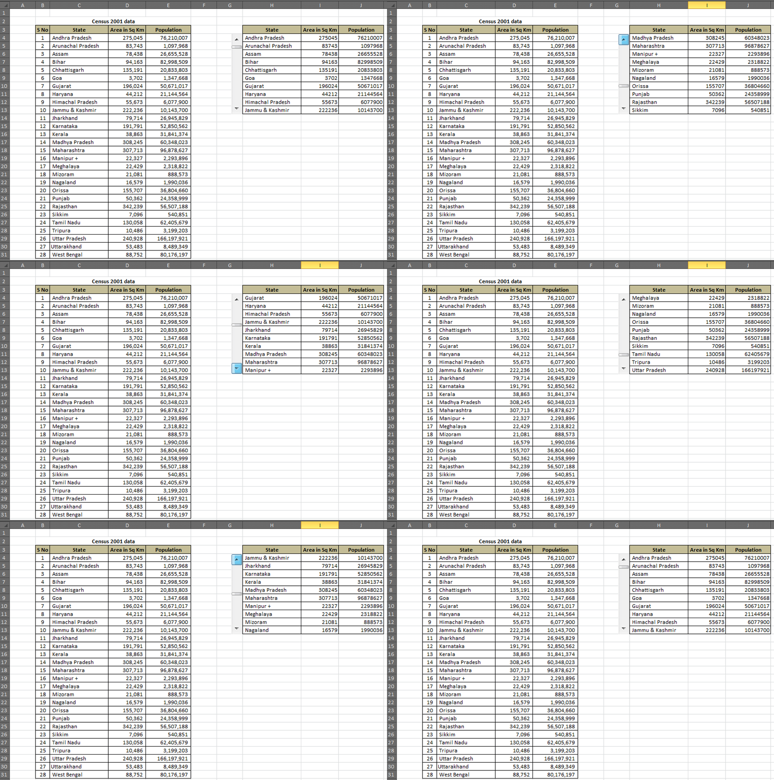
For the purpose of this tutorial, I have taken the data for 28 states in India, along with each state’s area and population (census 2001). Now, I want to create a data set that displays only 10 states at a time, and when the user changes the scroll bar, the data dynamically changes.
Something like this shown below:

Steps to Create a Scroll Bar in Excel
- The first step is to get your data in place. For the purpose of this post, I have used census 2001 data of 28 Indian States with its Area and Population.
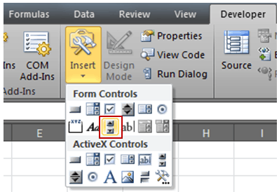
- Go to Developer Tab –> Insert –> Scroll Bar (Form Control).

- If you can’t find the developer tab in the ribbon, it is because it has not been enabled. By default, it’s hidden in Excel. You first need to add the developer tab in the ribbon.
- Click on Scroll Bar (Form Control) button and click anywhere on your worksheet. This will insert a Scroll Bar in the excel worksheet.
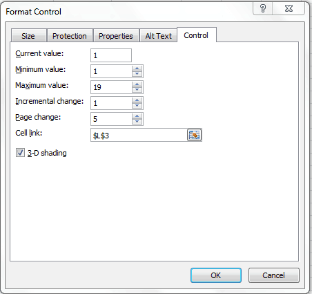
- Right-click on the Scroll Bar and click on ‘Format Control’. This will open a Format Control dialog box.
- In Format Control dialogue box go to the ‘Control’ tab, and make the following changes:
- Current Value: 1
- Minimum Value: 1
- Maximum Value: 19 (it is 19 here as we display 10 rows at a time. So when the user makes the scroll bar value 19, it displays rows 19-28)
- Incremental Change: 1
- Page Change: 5
- Cell Link: $L$3

$L$3 is the cell that is linked to the scroll bar in Excel. Its value varies from 1 to 19. This is the cell value that we use to make the scrollable list. Don’t worry if it doesn’t make sense as of now. Just keep reading and it will become clear!!
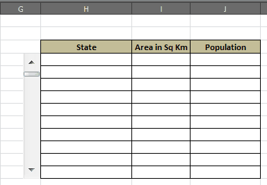
6. Resize the Scroll Bar so that it fits the length of the 10 columns (this is just to give it a good look, as shown in the pic below).

7. Now enter the following formula in the first cell (H4) and then copy it to fill all the other cells:
- =OFFSET(C3,$L$3,0)4
Note that this OFFSET formula is dependent on cell L3, which is linked to the scroll bar.
Now you are all set with a Scroll Bar in Excel.
How does this work?
The OFFSET formula uses cell C3 as the reference cell and offsets it by the values specified by cell L3. Since L3 is linked to scroll bar value, when the scrollbar value becomes 1, the formula refers to the first state name. When it becomes 2, it refers to the second state.
Also, since C3 cell has not been locked, in the second row, the formula becomes =OFFSET(C4,$L$3,0) and works the same way.
Dear Visitors, Please do write comments/issues if you have. we will try to resolve it.
No comments:
Post a Comment