MS Excel: How to use the IF Function
The IF function is one of the most popular and useful functions in Excel. You use an IF statement to ask Excel to test a condition and to return one value if the condition is met, and another value if the condition is not met.
In this tutorial, we are going to learn the syntax and common usages of Excel IF function, and then will have a closer look at formula examples that will hopefully prove helpful both to beginners and experienced Excel users.
- Excel IF function - syntax and usage
- Using the IF function in Excel - formula examples
- IF examples for numbers
- How to use the IF function with text values
- Using Excel IF function with dates
- Excel IF statement for blank, non-blank cells
Excel IF function - syntax and usage
The IF function is one of Excel's logical functions that evaluates a certain condition and returns the value you specify if the condition is TRUE, and another value if the condition is FALSE.
The syntax for Excel IF is as follows:
IF(logical_test, [value_if_true], [value_if_false])
As you see, the IF function has 3 arguments, but only the first one is obligatory, the other two are optional.
- logical_test (required) - a value or logical expression that can be either TRUE or FALSE. In this argument, you can specify a text value, date, number, or any comparison operator.For example, your logical test can be expressed as or B1="sold", B1<12/1/2014, B1=10 or B1>10.
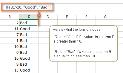
- value_if_true (optional) - the value to return when the logical test evaluates to TRUE, i.e. if the condition is met.For example, the following formula will return the text "Good" if a value in cell B1 is greater than 10:
=IF(B1>10, "Good") - value_if_false (optional) - the value to be returned if the logical test evaluates to FALSE, i.e. if the condition is not met.For example, if you add "Bad" as the third parameter to the above formula, it will return the text "Good" if a value in cell B1 is greater than 10, otherwise, it will return "Bad":
=IF(B1>10, "Good", "Bad")
Excel IF function - things to remember!
Though the last two parameters of the IF function are optional, your formula may produce unexpected results if you don't know the underlying logic beneath the hood.
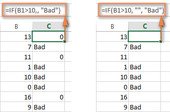
- If value_if_true is omittedIf the value_if_true argument is omitted in your Excel IF formula (i.e. there is only a comma following logical_test), the IF function returns zero (0) when the condition is met. Here is an example of such a formula:
=IF(B1>10,, "Bad")In case you don't want your Excel IF statement to display any value when the condition is met, enter double quotes ("") in the second parameter, like this:=IF(B1>10, "", "Bad"). Technically, in this case the formula returns an empty string, which is invisible to the user but perceivable to other Excel functions.The following screenshot demonstrates the above approaches in action, and the second one seems to be more sensible:
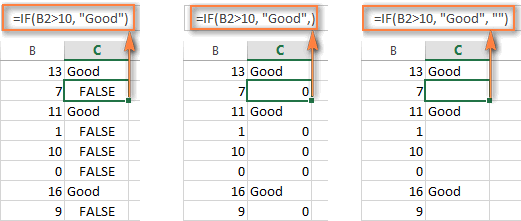
- If value_if_false is omittedIf you don't care what happens when the specified condition is not met, you can omit the 3rd parameter in your Excel IF formulas, which will result in the following.If the logical test evaluates to FALSE and the
value_if_falseparameter is omitted (there is just a closing bracket after thevalue_if_trueargument), the IF function returns the logical value FALSE. It's a bit unexpected, isn't it? Here is an example of such a formula:=IF(B1>10, "Good")Putting a comma after the value_if_true argument forces your IF statement to return 0, which doesn't make much sense either:=IF(B1>10, "Good",)And again, the most reasonable approach is to put "" in the third argument, in this case you will have empty cells when the condition is not met:=IF(B1>10, "Good", "")
- Get the IF function to display logical values TRUE or FALSEFor your Excel IF formula to display the logical values TRUE and FALSE when the specified condition is met and not met, respectively, type TRUE in the
value_if_trueargument. Thevalue_if_falseparameter can be FALSE or omitted. Here's a formula example:=IF(B1>10, TRUE, FALSE)
or
=IF(B1>10, TRUE)
 Note. For your Excel IF statement to return TRUE and FALSE as the logical values (Boolean values) that other Excel formulas can recognize, make sure you don't enclose them in double quotes. A visual indication of a Boolean is middle align in a cell, as you see in the screenshot above.
If you want "TRUE" and "FALSE" to be usual text values, enclose them in "double quotes". In this case, the returned values will be aligned left and formatted as General. No Excel formula will recognize such "TRUE" and "FALSE" text as logical values. - IF statement to perform a math operation and return a resultInstead of returning certain values, you can get your IF formula to test the specified condition, perform a corresponding math operation and return a value based on the result. You do this by using arithmetic operators or other Excel functions in the
value_if_trueand /orvalue_if_falsearguments. Here are just a couple of formula examples:Example 1:=IF(A1>B1, C3*10, C3*5)The formula compares the values in cells A1 and B1, and if A1 is greater than B1, it multiplies the value in cell C3 by 10, by 5 otherwise.Example 2:=IF(A1<>B1, SUM(A1:D1), "")The formula compares the values in cells A1 and B1, and if A1 is not equal to B1, the formula returns the sum of values in cells A1:D1, an empty string otherwise.
Using the IF function in Excel - formula examples
Now that you are familiar with the Excel IF function's syntax, let's look at some formula examples and learn how to use IF as a worksheet function in Excel.
Excel IF statement for numbers: greater than, less than, equal to
The use of the IF function with numeric values is based on using different comparison operators to express your conditions. You will find the full list of logical operators illustrated with formula examples in the table below.
| Condition | Operator | Formula Example | Description |
| Greater than | > | =IF(A2>5, "OK",) | If the number in cell A2 is greater than 5, the formula returns "OK"; otherwise 0 is returned. |
| Less than | < | =IF(A2<5, "OK", "") | If the number in cell A2 is less than 5, the formula returns "OK"; an empty string otherwise. |
| Equal to | = | =IF(A2=5, "OK", "Wrong number") | If the number in cell A2 is equal to 5, the formula returns "OK"; otherwise the function displays "Wrong number". |
| Not equal to | <> | =IF(A2<>5, "Wrong number", "OK") | If the number in cell A2 is not equal to 5, the formula returns "Wrong number "; otherwise - "OK". |
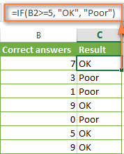
| Greater than or equal to | >= | =IF(A2>=5, "OK", "Poor") | If the number in cell A2 is greater than or equal to 5, the formula returns "OK"; otherwise - "Poor". |
| Less than or equal to | <= | =IF(A2<=5, "OK", "") | If the number in cell A2 is less than or equal to 5, the formula returns "OK"; an empty string otherwise. |
The screenshot below demonstrates the IF formula with the "Greater than or equal to" logical operator in action:

Excel IF function examples for text values
Generally, you write an Excel if statement with text using either "equal to" or "not equal to" operator, as demonstrated in a couple of IF examples that follow.
Example 1. Case-insensitive IF formula for text values
Like the overwhelming majority of Excel functions, IF is case-insensitive by default. What it means for you is that logical tests for text values do not recognize case in usual IF formulas.
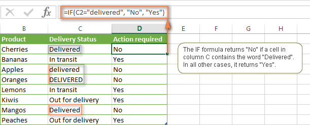
For example, the following IF formula returns either "Yes" or "No" based on the "Delivery Status" (column C):
=IF(C2="delivered", "No", "Yes")
Translated into plain English, the formula tells Excel to return "No" if a cell in column C contains the word "Delivered", otherwise return "Yes". At that, it does not really matter how you type the word "Delivered" in the logical_test argument - "delivered", "Delivered", or "DELIVERED". Nor does it matter whether the word "Delivered" is in lowercase or uppercase in the source table, as illustrated in the screenshot below.

Another way to achieve exactly the same result is to use the "not equal to" operator and swap the value_if_true and value_if_false arguments:
=IF(C2<>"delivered", "Yes", "No")Example 2. Case-sensitive IF formula for text values
If you want a case-sensitive logical test, use the IF function in combination with EXACT that compares two text strings and returns TRUE if the strings are exactly the same, otherwise it returns FALSE. The EXACT functions is case-sensitive, though it ignores formatting differences.
You use IF with EXACT in this way:
=IF(EXACT(C2,"DELIVERED"), "No", "Yes")
Where C is the column to which your logical test applies and "DELIVERED" is the case-sensitive text value that needs to be matched exactly.
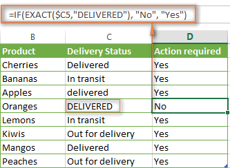

Naturally, you can also use a cell reference rather than a text value in the 2nd argument of the EXACT function, if you want to.
Note. When using text values as parameters for your IF formulas, remember to always enclose them in "double quotes".
Example 3. Excel if statement for text with partial match
If you want to base your condition on a partial match rather than exact match, an immediate solution that comes to mind is using wildcard characters (* or ?) in the logical_test argument. However, this simple and obvious approach won't work. Many Excel functions accept wildcards, but regrettably IF is not one of them.
A solution is to use IF in combination with ISNUMBER and SEARCH (case-insensitive) or FIND (case-sensitive) functions.
For example, if No action is required both for "Delivered" and "Out for delivery" items, the following formula will work a treat:
=IF(ISNUMBER(SEARCH("deliv",C2)), "No", "Yes")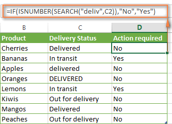
We've used the SEARCH function in the above formula since a case-insensitive match suits better for our data. If you want a case-sensitive match, simply replace SEARCH with FIND in this way:
=IF(ISNUMBER(FIND("text", where to search)), value_if_true, value_if_false)
Excel IF formula examples for dates
At first sight, it may seem that IF formulas for dates are identical to IF statements for numeric and text values that we've just discussed. Regrettably, it is not so.
Unlike many other Excel functions, IF cannot recognize dates and interprets them as mere text strings, which is why you cannot express your logical test simply as >"11/19/2014" or >11/19/2014. Neither of the above arguments is correct, alas.
Example 1. IF formulas for dates with DATEVALUE function
To make the Excel IF function recognize a date in your logical test as a date, you have to wrap it in the DATEVALUE function, like this DATEVALUE("11/19/2014"). The complete IF formula may take the following shape:
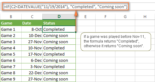
=IF(C2<DATEVALUE("11/19/2014"), "Completed", "Coming soon")
As illustrated in the screenshot below, this IF formula evaluates the dates in column C and returns "Completed" if a game was played before Nov-11. Otherwise, the formula returns "Coming soon".

Example 2. IF formulas with TODAY() function
In case you base your condition on the current date, you can use the TODAY() function in the logical_test argument of your IF formula. For example:
=IF(C2<DATEVALUE("11/19/2014"), "Completed", "Coming soon")
Naturally, the Excel IF function can understand more complex logical tests, as demonstrated in the next example.
Example 3. Advanced IF formulas for future and past dates
Suppose, you want to mark only the dates that occur in more than 30 days from now. In this case, you can express the logical_test argument as A2-TODAY()>30. The complete IF formula may be as follows:
=IF(A2-TODAY()>30, "Future date", "")
To point out past dates that occurred more than 30 days ago, you can use the following IF formula:
=IF(TODAY()-A2>30, "Past date", "")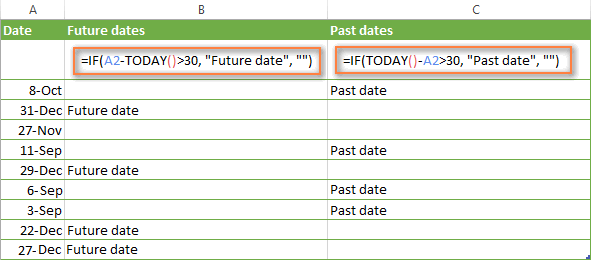
If you want to have both indications in one column, you will need to use a nested IF function like this:
=IF(A2-TODAY()>30, "Future date", IF(TODAY()-A2>30, "Past date", ""))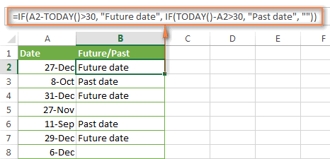
Excel IF examples for blank, non-blank cells
If you want to somehow mark your data based on a certain cell(s) being empty or not empty, you can either:
- Use the Excel IF function in conjunction with ISBLANK, or
- Use the logical expressions ="" (equal to blank) or <>"" (not equal to blank).
The table below explains the difference between these two approaches and provides formula example.
| Logical test | Description | Formula Example | |
| Blank cells | ="" | Evaluates to TRUE if a specified cell is visually empty, including cells with zero length strings.
Otherwise, evaluates to FALSE.
| =IF(A1="", 0, 1)
Returns 0 if A1 is visually blank. Otherwise returns 1.
If A1 contains an empty string, the formula returns 0.
|
| ISBLANK() | Evaluates to TRUE is a specified cell contains absolutely nothing - no formula, no empty string returned by some other formula.
Otherwise, evaluates to FALSE.
| =IF(ISBLANK(A1), 0, 1)
Returns the results identical to the above formula but treats cells with zero length strings as non-blank cells.
That is, if A1 contains an empty string, the formula returns 1.
| |
| Non-blank cells | <>"" | Evaluates to TRUE if a specified cell contains some data. Otherwise, evaluates to FALSE.
Cells with zero length strings are considered blank.
| =IF(A1<>"", 1, 0)
Returns 1 if A1 is non-blank; otherwise returns 0.
If A1 contains an empty string, the formula returns 0.
|
| ISBLANK()=FALSE | Evaluates to TRUE if a specified cell is not empty. Otherwise, evaluates to FALSE.
Cells with zero length strings are considered non-blank.
| =IF(ISBLANK(A1)=FALSE, 0, 1)
Works the same as the above formula, but returns 1 if A1 contains an empty string.
|
The following example demonstrates blank / non-blank logical test in action.
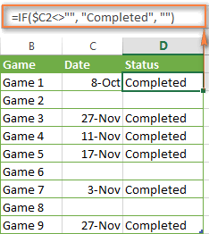
Suppose, you have a date in column C only if a corresponding game (column B) was played. Then, you can use either of the following IF formulas to mark completed games:
=IF($C2<>"", "Completed", "")=IF(ISBLANK($C2)=FALSE, "Completed", "")
Since there are no zero-length strings in our table, both formulas will return identical results:

Hopefully, the above examples have helped you understand the general logic of the IF function. In practice, however, you would often want a single IF formula to check multiple conditions, and our next article will show you how to tackle this task. In addition, we will also explore nested IF functions, array IF formulas, IFEFFOR and IFNA functions and more. Please stay tuned and thank you for reading!
Dear Visitors, Please do write comments/issues if you face any. I will try to resolve it.
